Comprehensive Comparison of Dimensionality Reduction Methods

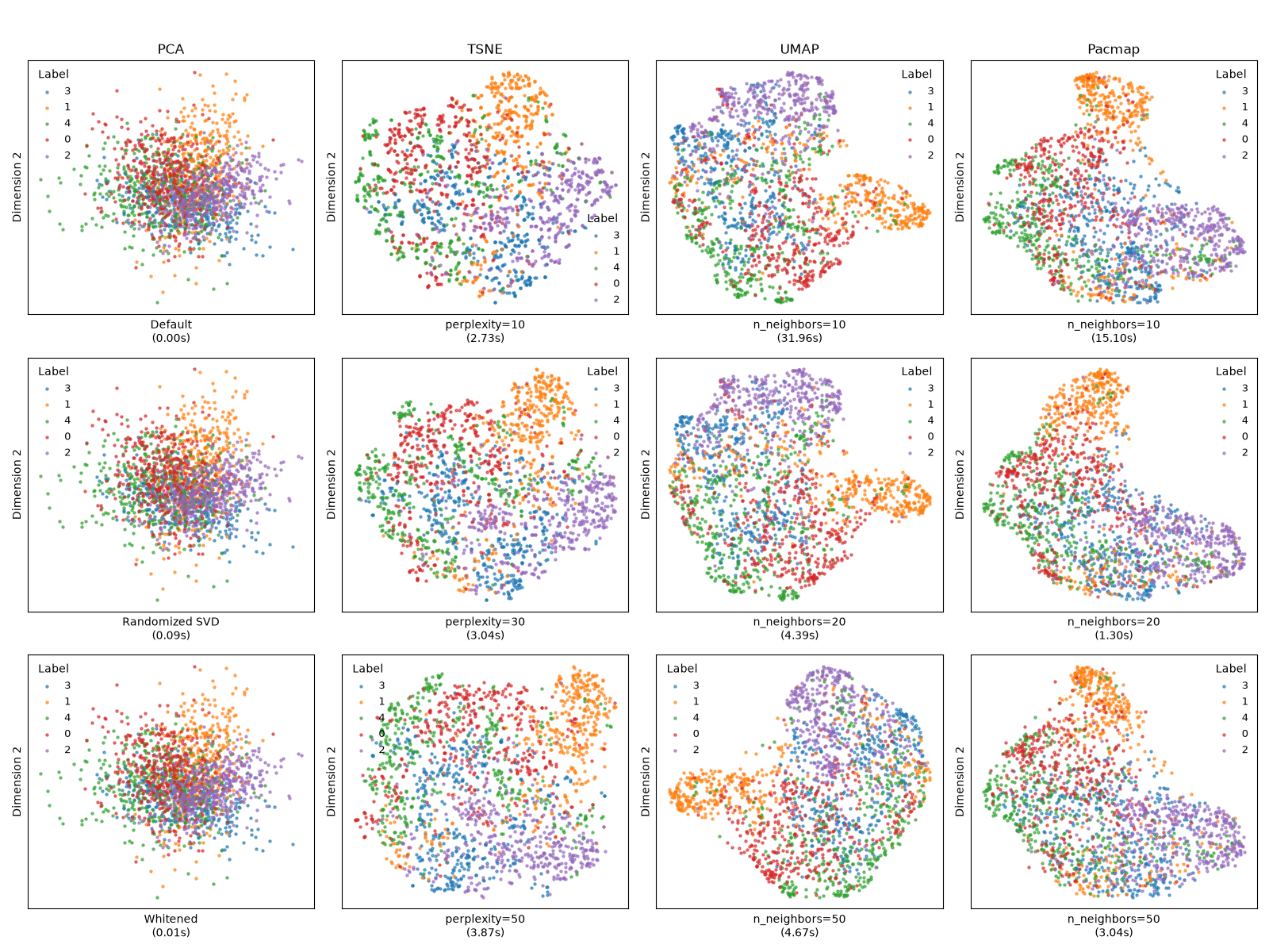
This example compares several dimensionality reduction algorithms (PCA, t-SNE, UMAP, and Pacmap) across different parameter settings using a synthetic high-dimensional dataset. It demonstrates how hyperparameter choices can drastically affect the resulting embeddings.

Imports and Setup

import os
import time
import warnings

import matplotlib.pyplot as plt
from sklearn.datasets import make_classification

from coco_pipe.dim_reduction import DimReduction
from coco_pipe.viz.dim_reduction import plot_embedding

# Prevent multiprocessing segfaults on macOS by limiting threads
os.environ["OMP_NUM_THREADS"] = "1"
os.environ["LOKY_MAX_CPU_COUNT"] = "1"
os.environ["NUMEXPR_MAX_THREADS"] = "1"

# Suppress warnings for cleaner output
warnings.filterwarnings("ignore")

1. Generate Synthetic Data

We create a synthetic dataset with 5 distinct classes embedded in a 50-dimensional space to simulate a complex, high-dimensional classification problem.

n_samples = 2000
n_features = 50
n_classes = 5

X, y = make_classification(
    n_samples=n_samples,
    n_features=n_features,
    n_informative=10,
    n_redundant=10,
    n_classes=n_classes,
    n_clusters_per_class=1,
    random_state=42,
)

print(f"Dataset shape: {X.shape}")
print(f"Number of classes: {n_classes}")

Dataset shape: (2000, 50)
Number of classes: 5

2. Define Methods and Parameters

We will test PCA, t-SNE, UMAP, and Pacmap, varying key parameters like perplexity or number of neighbors to observe their effect on the resulting topology.

method_params = {
    "PCA": [
        ({}, "Default"),
        ({"svd_solver": "randomized"}, "Randomized SVD"),
        ({"whiten": True}, "Whitened"),
    ],
    "TSNE": [
        ({"perplexity": 10, "max_iter": 500}, "perplexity=10"),
        ({"perplexity": 30, "max_iter": 500}, "perplexity=30"),
        ({"perplexity": 50, "max_iter": 500}, "perplexity=50"),
    ],
    "UMAP": [
        ({"n_neighbors": 10, "min_dist": 0.1}, "n_neighbors=10"),
        ({"n_neighbors": 20, "min_dist": 0.1}, "n_neighbors=20"),
        ({"n_neighbors": 50, "min_dist": 0.1}, "n_neighbors=50"),
    ],
    "Pacmap": [
        ({"n_neighbors": 10}, "n_neighbors=10"),
        ({"n_neighbors": 20}, "n_neighbors=20"),
        ({"n_neighbors": 50}, "n_neighbors=50"),
    ],
}

3. Compute Embeddings

We iterate over the methods and their parameter sets, computing the 2D embedding and recording the elapsed time.

results = {method: [] for method in method_params}

for method, param_sets in method_params.items():
    print(f"Evaluating {method}...")
    for params, param_str in param_sets:
        reducer = DimReduction(method=method, n_components=2, **params)

        start_time = time.time()
        X_reduced = reducer.fit_transform(X)
        elapsed = time.time() - start_time

        results[method].append((X_reduced, param_str, elapsed))

Evaluating PCA...
Evaluating TSNE...
Evaluating UMAP...
Evaluating Pacmap...

4. Visualize Grid Comparison

We plot the resulting embeddings in a grid, where columns represent methods and rows represent different parameter settings.

methods = [m for m in method_params if len(results[m]) > 0]
n_methods = len(methods)
n_params = max(len(results[m]) for m in methods)

fig, axes = plt.subplots(n_params, n_methods, figsize=(n_methods * 4, n_params * 4))

for col, method in enumerate(methods):
    method_results = results[method]
    for row, (X_red, param_str, elapsed) in enumerate(method_results):
        ax = axes[row, col]

        # Use our viz module to plot the embedding
        plot_embedding(
            X_red,
            labels=y,
            ax=ax,
            s=5,
            alpha=0.6,
            palette="tab10",
            title=f"{method}" if row == 0 else "",
            label_kind="categorical",
        )

        ax.set_xlabel(f"{param_str}\n({elapsed:.2f}s)", fontsize=10)
        ax.set_xticks([])
        ax.set_yticks([])

# Fill empty subplots if any
for method in methods:
    n_results = len(results[method])
    for row in range(n_results, n_params):
        axes[row, methods.index(method)].axis("off")

plt.suptitle("Dimension Reduction Methods Comparison", fontsize=18, y=1.02)
plt.tight_layout()
plt.show()

Conclusion

This comprehensive comparison illustrates that:

1. PCA provides a rapid baseline but struggles to separate complex non-linear structures. 2. t-SNE creates beautiful, distinct clusters but is highly sensitive to the perplexity parameter and takes longer to compute. 3. UMAP effectively balances local and global structure preservation while remaining computationally efficient. 4. Pacmap aims to preserve both local and global structures simultaneously, often rivaling UMAP in speed and cluster quality.